Author: Jethro Johnson
Contributors:
Updated: 11 May 2020

DADA2: Improving Taxonomic Resolution

Introduction

Clustering 16S sequences into OTUs has historically served two purposes:

It has removed minor artifactual sequence variants due to PCR amplification and sequencing errors.
It has collapsed legitimate sequence variation that exists between closely related bacterial taxa.

While the latter may not always be desirable, it stands to reason that you can’t distinguish between bacterial taxa whose 16S sequences vary at a rate that is lower than the error encountered on a particular sequencing platform.

Recently, a number of tools have been developed with the goal of removing PCR and sequencing errors in 16S data (‘denoising’). Examples include Minimum entropy decomposition, UNOISE, DADA2, and Deblur. For a recent comparison of some of these tools, see here.

These approaches collectively claim it is now possible to distinguish between sequences that differ by as little as one nucleotide. In consequence, they argue that denoised sequences (variously called exact sequence variants (ESVs), amplicon sequence variants (ASVs), or zero-radius OTUs (ZOTUs)) should replace conventional OTUs as the unit of measurement in 16S studies.

While the main practical session is focused on conventional OTU analysis. This session contains an introduction to sequence analysis based on the DADA2 pipeline.

  1. Fetching Data for DADA2 Analysis
  2. Open DADA2 and Plot Read Quality
  3. Trim and filter forward and reverse reads based on quality
  4. Denoise reads with DADA2
  5. Genererate amplicons and create an abundance matrix
  6. Assign Taxonomy to DADA2 Amplicon Sequence Variants

Conlusions

1. Fetching Data for DADA2 Analysis

For this session we’ll use a slightly different set of input samples. Start by creating a run directory and copying the data to this location.

# Create a working directory for this session
cd ~/MCA/16s/
mkdir Session1.3
mkdir Session1.3/fastqs
cd Session1.3/fastqs

# Copy the fastq files for three samples to this location
cp ~/additional_data/sample* .

# Note these files are gzip compressed, but it is still possible to view them
# using the linux pipe.
zcat sample1_trimmed.fastq.1.gz | head -4

2. Open DADA2 and Plot Read Quality

As the DADA2 package is written entirely in R, most of this session will be carried out in RStudio.

Nagivate to your RStudio session and open a new R script.

RStudio

Remember, you can write (and comment!) code in your new R script then run it via the R terminal, either by copying and pasting it across, or by highlighting it and selecting the Run icon in the top-right side of your script window.

RStudio

Having opened RStudio, set your working directory to be the location of the run directory created in step 1.

# Find out which working directory R is running in?
getwd()

# Set your working directory and check the contents
setwd('~/MCA/16s/Session1.3')
list.files('.')
list.files('./fastqs')

Note that the fastq files have been trimmed to remove PCR and sequencing primers. However, they have not been trimmed to remove low quality sequences at the 3’ end of reads. We will use the DADA2 function plotQualityProfile() to visualize the distribution in quality at each base in the forward and reverse reads from the first sample.

# Create avectors in R containing details of forward and reverse reads
fastq1 <- sort(list.files('fastqs', pattern='.fastq.1.gz', full.names=T))
fastq2 <- sort(list.files('fastqs', pattern='.fastq.2.gz', full.names=T))

# Plot the read quality distribution for each sample pair
plotQualityProfile(c(fastq1, fastq2))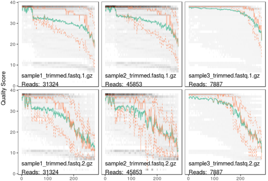

RStudio

In this plot lines show the mean (green), median (orange) and 25th/75th percentiles (dashed) of the quality score at each base position in the forward and reverse reads.

A side note on handling data with R

When working on the bash command line, we have tended to use for loops to run the same command for multiple samples. R is not optimised for running for loops and it takes a fundamentally different approach. For further discussion of why this is have a look at the family of apply functions in R, as well as the fundamentals of the split-apply-combine stragegy.

For the purposes of this practical session note that, rather than using a for loop to run plotQualityProfile() above, we passed all the files to the function as a single character vector. This is typical of how R deals with repetitive tasks.

3. Trim and filter forward and reverse reads based on quality

The first step in processing reads with DADA2 is to remove poor quality sequence. In our main 16S analysis session this step wasn’t performed. Instead we were relying on the FLASh assembler and downstream OTU calling to account for low quality sequence.

Similar to our bash code, it’s necessary to define the names of input and output files before running the filtering step.

# Create a subdirectory from within R to contain quality trimmed sequences
dir.create('fastqs_trimmed')

# This subdirectory now appears in your working directory
list.files('.')
list.files('./fastqs_trimmed')

# Fetch a list of sample names from the list of forward reads
sample.names <- sapply(strsplit(basename(fastq1), '_'), `[`, 1)

# Create vectors of output filenames for both forward and reverse reads
fastq1.filtered <- file.path('fastqs_trimmed', paste0(sample.names, '.fastq.1.gz'))
fastq2.filtered <- file.path('fastqs_trimmed', paste0(sample.names, '.fastq.2.gz'))

# Run quality trimming and filtering in DADA2
out <- filterAndTrim(fwd=fastq1, filt=fastq1.filtered,
       		     rev=fastq2, filt.rev=fastq2.filtered,
                     truncLen=c(260, 260),
		     maxEE=c(2,2),
                     multithread=T)

list.files('./fastqs_trimmed')
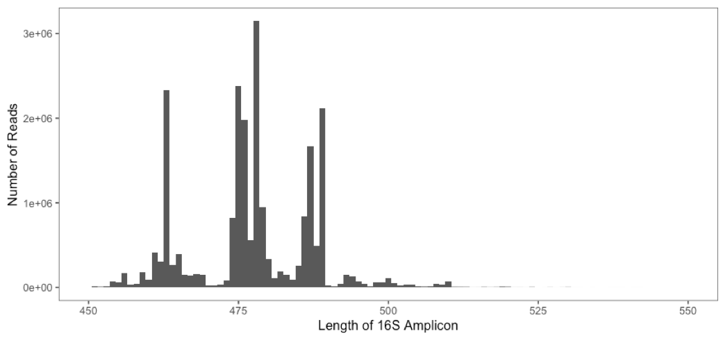
print(out)

In the code above, we’ve set the minimum permissible truncated length of for a sequence to be 260bp for both forward and reverse reads. These were originally 2x300bp reads generated on the Illumina MiSeq platform to span the (~500bp) V1-V3 region. However, 20bp has been trimmed from the 5’ end of each read during adapter removal. This minimum lengths used above have therefore been selected to ensure (minimal!) overlap between reads during amplicon assembly.

The histogram below shows a typical distribution in the length of amplicons generated from a human gut microbiome study.

RStudio

What biases may be introduced by setting a stringent truncLen value?

For more information on the arguments supplied in the quality trimming and filtering step type ?filterAndTrim into the R terminal.

Try altering truncLen and replacing maxEE with a minimum quality score (minQ) to see what effect these parameters have on the number of reads remaining after filtering.

4. Denoise reads with DADA2

Denoising in DADA2 is a two step process, first it models the expected error the forward and reverse reads, then it removes this error to create a ‘corrected’ read set. For further detail see the methods and supplementary material in the original DADA2 publication.

# Model error in forward and reverse reads
error1 <- learnErrors(fastq1.filtered)
error2 <- learnErrors(fastq2.filtered)

# Remove exact replicate sequences
dereplicated1 <- derepFastq(fastq1.filtered, verbose=T)
names(dereplicated1) <- sample.names
dereplicated2 <- derepFastq(fastq2.filtered, verbose=T)
names(dereplicated2) <- sample.names

# Then apply the DADA2 denoising algorithm
corrected1 <- dada(dereplicated1, err=error1)
corrected2 <- dada(dereplicated2, err=error2)

corrected1
corrected2

5. Genererate amplicons and create an abundance matrix

Having corrected sequencing errors in forward and reverse reads, the remaining steps are to merge read pairs into amplicons, remove chimeras, and to calculate the abundance of each amplicon in each sample.

# Combine the forward and reverse read into a single set of amplicons
amplicons <- mergePairs(dadaF=corrected1, derepF=dereplicated1,
                        dadaR=corrected2, derepR=dereplicated2,
                        verbose=T)

# Generate a count matrix containing the counts for each denoised sequence
sequence.tab <- makeSequenceTable(amplicons, orderBy='abundance')

# The rows of this matrix are the samples
rownames(sequence.tab)
# The columns are the sequences
colnames(sequence.tab)

# Remove chimeras directly from the count.matrix
sequence.tab.nochimeras <- removeBimeraDenovo(sequence.tab, verbose=T)

# Finally, it's possible to write the denoised amplicons to a fasta file
uniquesToFasta(getUniques(sequence.tab.nochimeras), 'dada2_esvs.fasta')

How many unique amplicons were created using the DADA2 denoising pipeline?

6. Assign Taxonomy to DADA2 Amplicon Sequence Variants

Within the DADA2 pipeline, it is also possible to assign taxonomy to denoised sequences via a two step process. The first step assignTaxonomy() is a wrapper for the method introduced in our previous 16 analysis session. As this method only returns classifications to genus level. The second step addSpecies() attempts to find exact matches for each sequence in a curated reference database.

First, it’s necessary to retrieve the reference databases for taxonomic and species assignment. A selection of formatted reference databases can be found here. In this example we will begin by downloading reference databases derived from the NCBI 16S database and the RDP database.

# In your bash terminal cd into the current working directory
cd ~/MCA/16s/Session1.3

# Download the database used to train the RDP classifier
curl -O -J -L https://zenodo.org/record/2541239/files/RefSeq-RDP16S_v2_May2018.fa.gz?download=1
# Download the database used for exact sequence matching
curl -O -J -L https://zenodo.org/record/2658728/files/RefSeq-RDP_dada2_assignment_species.fa.gz?download=1

ls -l

Having downloaded the reference databases, return to R to perform taxonomic assignment.

# Assign taxonomy to genus level
taxonomy.table <- assignTaxonomy(seqs=sequence.tab.nochimeras,
                       refFasta="RefSeq-RDP16S_v2_May2018.fa.gz",
                       multithread=T)
# Assign species via exact matching
taxonomy.table <- addSpecies(taxtab=taxonomy.table,
                             refFasta="RefSeq-RDP_dada2_assignment_species.fa.gz",
                             verbose=T)

# As row names in the resulting table are the sequences
# remove them before viewing.
taxa.print <- taxa
row.names(taxa.print) <- NULL
taxa.print <- as.data.frame(taxa.print)
View(taxa.print)

Alternatively, it is possible to assign taxonomy to the denoised amplicon sequences by using the NCBI nucleotide BLAST tool. This can be done by copying and pasting individual sequences into the online BLAST portal. Then selecting the highly-curated NCBI 16S rRNA database as a reference.

BLAST

Try running BLAST for the most and least abundant ASVs in your output fasta file.

Try running BLAST against the NCBI Nucleotide collection database, rather than the 16S rRNA database.

Note that it’s also possible to install BLAST locally and run it from the commandline. However, if you do this, for taxonomic assignment, be very careful about the arguments you provide.

Conclusions

DADA2 and other denoising algorithms provide a different approach to dealing with sequencing error compared to more traditional OTU-based analysis.

In OTU analysis sequencing error is removed by collapsing sequences at an identity threshold that is (hopefully!) higher than the error rate encountered on a particular sequencing platform. DADA2 models this error before removing it from each (unique) sequence.

Both approaches have strengths and weaknesses. Proponents of denoising algorithms argue that they have two major theoretical advantages:

First, they remove the need to collapse legitimate sequence variation that may occur between closely related taxa. This enables finer taxonomic resolution in 16S studies.
Second, the ability to identify exact sequences means sequences can be compared across studies. By contrast, the manner in which OTUs are generated means they are unique to the study in which they are derived.

While these are significant advantages, biological judgement is required when interpreting denoised amplicon data. For example, how many of the denoised amplicon sequences could confidently be classified to species level? To what extent does this depend on the completness and accuracy of the 16S rRNA reference databases?

Another interesting point to consider is that the three samples analyzed in this session were drawn from a mock community made up of 36 bacterial species. The list of included species is given below:


Actinomyces naeslundii MG-1	Akkermansia muciniphila	Bacteroides caccae
Bacteroides vulgatus	Bifidobacterium dentium	Bifidobacterium longum subsp. infantis
Corynebacterium accolens	Corynebacterium amycolatum	Corynebacterium matruchotti
Enterococcus faecalis	Escherichia coli	Eubacterium brachy
Faecalibacterium prausnitzii	Fusobacterium nucleatum subsp. nucleatum	Gardnerella vaginalis
Lactobacillus crispatus	Lactobacillus gasseri	Lactobacillus iners
Lactobacillus jensenii	Lautropia mirabilis	Moraxella catarrhalis
Porphyromonas gingivalis	Prevotella melaninogenica	Prevotella nigrescens
Prevotella oralis	Propionibacterium acnes	Rothia dentocariosa
Ruminococcus lactaris	Staphylococcus aureus subsp. aureus	Streptococcus agalactiae
Streptococcus mutans	Streptococcus pneumoniae	Streptococcus sanguinis
Tannerella forsythia	Treponema denticola	Veillonella parvula

How many ASVs were generated by DADA2 compared to the number of species in this community?

How many of the species above were identified by the different taxonomic classification approaches?

What happens when you run these three samples through the OTU pipeline introduced in the main session?

What happens when you increase the identity threshold used for OTU clustering from 97% to 99%?

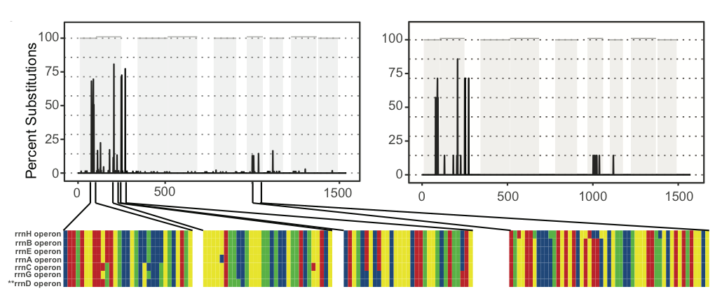
One final point to consider when interpreting ASVs is that many bacteria contain multiple copies of the 16S gene that may vary in their sequence composition. The image below shows the observed (left) and predicted (right) frequency of nucleotide substitutions occurring across the seven (~1500bp) 16S genes present in the genome of Escherichia coli strain K-12 subst. MG1655. In total five of these seven 16S genes are unique, while the remaining two are identical.

Ecoli

How many E. coli ASVs were detected by DADA2?